Getting Started with Kompot¶

This tutorial introduces Kompot’s core functionality for differential analysis in single-cell data. You’ll learn how to:

Perform differential abundance (DA) analysis to identify cell states that change between conditions
Conduct differential expression (DE) analysis to find genes with altered expression
Visualize and interpret results using Kompot’s plotting tools

What Makes Kompot Different?¶

Kompot uses Mahalanobis distance to detect expression differences while accounting for the covariance structure of gene expression. This approach is particularly powerful for:

Detecting subtle changes along continuous cell state trajectories
Identifying genes with complex, coordinated expression patterns
Analyzing data where discrete cell type labels are inadequate

Dataset¶

We’ll analyze murine bone marrow cells comparing Young vs. Old mice to understand how aging affects hematopoietic stem cells and their derivatives.

[1]:

import anndata as ad
import matplotlib.pyplot as plt
import numpy as np
import palantir
import pandas as pd
import scanpy as sc
import seaborn as sns

import kompot

# Set plotting style
plt.rcParams["axes.spines.right"] = False
plt.rcParams["axes.spines.top"] = False
plt.rcParams["image.cmap"] = "Spectral_r"

Configuration¶

Define analysis parameters. Adapt these to your own data:

[2]:

DATA_PATH = "../data/murine_bone_marrow_aging.h5ad"
GROUPING_COLUMN = "Age"              # Condition column in adata.obs
CONDITIONS = ["Young", "Old"]        # First condition is reference
CELL_TYPE_COLUMN = "highres_celltype"  # Optional: for visualization only
DIMENSIONALITY_REDUCTION = "DM_EigenVectors"  # Cell state representation
LAYER_FOR_EXPRESSION = "logged_counts"        # Expression data layer

Load Data¶

The dataset will be downloaded automatically from Zenodo if not already present:

[3]:

import os
from pathlib import Path
import requests
from tqdm.auto import tqdm

Path(DATA_PATH).parent.mkdir(parents=True, exist_ok=True)

if not os.path.exists(DATA_PATH):
    print("Downloading dataset...")
    url = "https://zenodo.org/records/15587768/files/murine_bone_marrow_aging.h5ad?download=1"
    response = requests.get(url, stream=True)
    total = int(response.headers.get("content-length", 0))

    with open(DATA_PATH, "wb") as file, tqdm(total=total, unit="B", unit_scale=True) as bar:
        for chunk in response.iter_content(chunk_size=8192):
            file.write(chunk)
            bar.update(len(chunk))

adata = ad.read_h5ad(DATA_PATH)
adata

[3]:

AnnData object with n_obs × n_vars = 8090 × 16285
    obs: 'Compartment', 'Replicate', 'Age', 'Sample', 'Info', 'batch', 'doublet_score', 'n_genes_by_counts', 'total_counts', 'total_counts_mt', 'pct_counts_mt', 'total_counts_hb', 'pct_counts_hb', 'S_score', 'G2M_score', 'phase', 'leiden', 'phenograph', 'highres_celltype', 'midres_celltype'
    var: 'gene_ids', 'feature_types', 'genome', 'mt', 'n_cells_by_counts', 'mean_counts', 'pct_dropout_by_counts', 'total_counts', 'hb', 'highly_variable', 'means', 'dispersions', 'dispersions_norm', 'highly_variable_nbatches', 'highly_variable_intersection'
    uns: 'Age_colors', 'Compartment_colors', 'DMEigenValues', 'Info_colors', 'README', 'Replicate_colors', 'Sample_colors', 'batch_colors', 'draw_graph', 'highres_celltype_colors', 'hvg', 'leiden', 'leiden_colors', 'midres_celltype_colors', 'neighbors', 'pca', 'phase_colors', 'umap'
    obsm: 'AbCapture', 'DM_EigenVectors', 'HTO', 'X_draw_graph_fa', 'X_pca', 'X_pca_harmony', 'X_pca_noregression', 'X_umap'
    varm: 'PCs'
    layers: 'MAGIC_imputed_data', 'logged_counts', 'normalized_counts', 'raw_counts'
    obsp: 'DM_Kernel', 'connectivities', 'distances'

Data Exploration¶

Before analysis, examine the data structure and distribution:

[4]:

sc.pl.umap(adata, color=[CELL_TYPE_COLUMN, GROUPING_COLUMN], frameon=False, wspace=1.3)

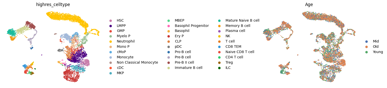
../_images/notebooks_01_getting_started_7_0.png

If you have a clustering or cell-type annotation, cell type composition can provide a rough understanding of the data and help identify underrepresented cell types that could complicate differential expression analysis.

[5]:

crosstab = (
    pd.crosstab(
        adata.obs[CELL_TYPE_COLUMN], adata.obs[GROUPING_COLUMN], normalize="index"
    )
    * 100
)

# Plot the distribution
ax = crosstab.plot(kind="bar", stacked=False, figsize=(12, 8))
ax.grid(False)
plt.xlabel("Cell Type")
plt.ylabel("Percentage (%)")
plt.title("Cell Type Distribution by Condition")
plt.legend(title=GROUPING_COLUMN)
plt.xticks(rotation=90)
plt.tight_layout()
plt.show()

# Print extremes (cell types with high bias toward one condition)
bias_threshold = 75  # Percentage threshold for considering a cell type biased
biased_types = crosstab[(crosstab > bias_threshold).any(axis=1)]

if not biased_types.empty:
    print(f"Cell types with >={bias_threshold}% bias toward one condition:")
    print(biased_types)
    print("\nThese cell types might show disproportionate changes between conditions.")

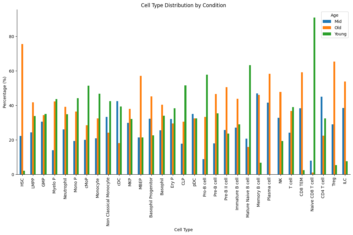
../_images/notebooks_01_getting_started_9_0.png

Cell types with >=75% bias toward one condition:
Age                     Mid        Old      Young
highres_celltype
HSC               22.257053  75.548589   2.194357
Naive CD8 T cell   8.000000   1.000000  91.000000

These cell types might show disproportionate changes between conditions.

Diffusion Maps Preprocessing¶

Kompot requires a continuous representation of cell states. Palantir diffusion maps capture the geometry of differentiation trajectories while reducing noise:

[6]:

palantir.utils.run_diffusion_maps(adata, pca_key="X_pca_harmony", n_components=40);

/fh/fast/setty_m/user/dotto/kompot/.venv/lib/python3.12/site-packages/joblib/externals/loky/backend/context.py:131: UserWarning: Could not find the number of physical cores for the following reason:
found 0 physical cores < 1
Returning the number of logical cores instead. You can silence this warning by setting LOKY_MAX_CPU_COUNT to the number of cores you want to use.
  warnings.warn(
  File "/fh/fast/setty_m/user/dotto/kompot/.venv/lib/python3.12/site-packages/joblib/externals/loky/backend/context.py", line 255, in _count_physical_cores
    raise ValueError(f"found {cpu_count_physical} physical cores < 1")

Differential Abundance Analysis¶

Identify cell states that change in frequency between conditions.

See kompot.da for full documentation.

[7]:

da_results = kompot.da(
    adata,
    groupby=GROUPING_COLUMN,
    condition1=CONDITIONS[0],
    condition2=CONDITIONS[1],
    obsm_key=DIMENSIONALITY_REDUCTION,
)

[2026-03-26 05:05:44,501] [INFO    ] Condition 1 (Young): 2,917 cells
[2026-03-26 05:05:44,502] [INFO    ] Condition 2 (Old): 3,116 cells
[2026-03-26 05:05:44,506] [INFO    ] Fitting density estimator for condition 1...
[2026-03-26 05:06:09,199] [INFO    ] Fitting density estimator for condition 2...
[2026-03-26 05:06:26,116] [INFO    ] This run will have `run_id=0`.

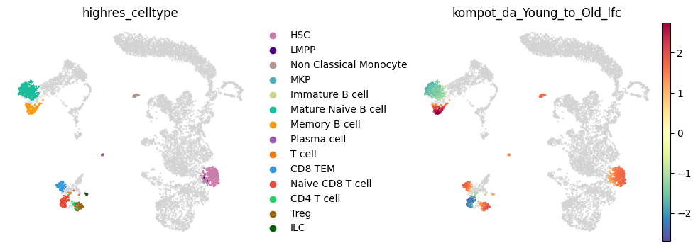
Visualize Abundance Changes¶

Results are stored in adata.obs:

kompot_da_Young_to_Old_lfc: Log fold change (positive = enriched in Old)
kompot_da_Young_to_Old_lfc_direction: Categorical classification (up/down/unchanged)

[8]:

sc.pl.embedding(
    adata, "umap",
    color=[f"kompot_da_{CONDITIONS[0]}_to_{CONDITIONS[1]}_lfc_direction", f"kompot_da_{CONDITIONS[0]}_to_{CONDITIONS[1]}_lfc"],
    color_map="RdBu_r",
    vcenter=0,
    frameon=False,
)

../_images/notebooks_01_getting_started_15_0.png

Volcano Plot¶

Volcano plots for differential abundance show effect size (x-axis) vs. statistical significance (y-axis):

[9]:

kompot.plot.volcano_da(adata, color=CELL_TYPE_COLUMN)

[2026-03-26 05:06:26,496] [INFO    ] Found DA run info for run_id=-1
[2026-03-26 05:06:26,497] [INFO    ] Found lfc_key='kompot_da_Young_to_Old_lfc' from run info
[2026-03-26 05:06:26,498] [INFO    ] Found ptp_key='kompot_da_Young_to_Old_neg_log10_lfc_ptp' from run info
[2026-03-26 05:06:26,500] [INFO    ] Successfully inferred fields: {'lfc_key': 'kompot_da_Young_to_Old_lfc', 'ptp_key': 'kompot_da_Young_to_Old_neg_log10_lfc_ptp'}
[2026-03-26 05:06:26,500] [INFO    ] Using inferred thresholds - lfc_threshold: 1.0, ptp_threshold: 0.05

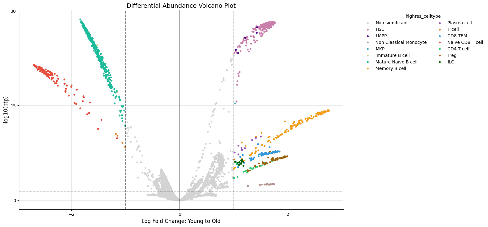
../_images/notebooks_01_getting_started_17_1.png

Points above the horizontal line and outside vertical lines are significantly changed.

Adjust thresholds using ptp_threshold and lfc_threshold parameters. Use update_direction=True to update the classification in adata.obs.

[10]:

# Visualize only significantly changed cells
kompot.plot.embedding(
    adata, "umap",
    color=[CELL_TYPE_COLUMN, f"kompot_da_{CONDITIONS[0]}_to_{CONDITIONS[1]}_lfc"],
    groups={f"kompot_da_{CONDITIONS[0]}_to_{CONDITIONS[1]}_lfc_direction": ["up", "down"]},
    frameon=False,
    wspace=.5,
)

[2026-03-26 05:06:27,096] [INFO    ] Selected 1,075 cells out of 8,090 total cells.

../_images/notebooks_01_getting_started_19_1.png

The mgroups parameter in the kompot.plot.embedding function allows plotting increasing and decreasing cell types separately:

[11]:

kompot.plot.embedding(
    adata,
    "umap",
    color=CELL_TYPE_COLUMN,
    mgroups=[{f"kompot_da_{CONDITIONS[0]}_to_{CONDITIONS[1]}_lfc_direction":[d]} for d in ["up", "down"]],
    frameon=False,
    wspace=.5,
)

[2026-03-26 05:06:27,853] [INFO    ] Selected 585 cells out of 8,090 total cells.
[2026-03-26 05:06:27,952] [INFO    ] Selected 490 cells out of 8,090 total cells.

../_images/notebooks_01_getting_started_21_1.png

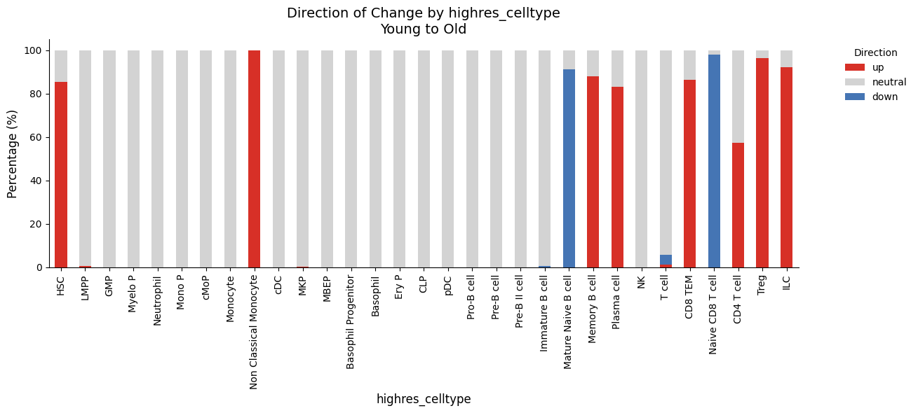
Summary by Cell Type¶

Aggregate abundance changes by cell type with the direction_barplot:

[12]:

kompot.plot.direction_barplot(adata, category_column=CELL_TYPE_COLUMN)

[2026-03-26 05:06:28,529] [INFO    ] Found DA run info for run_id=-1
[2026-03-26 05:06:28,530] [INFO    ] Found direction_key='kompot_da_Young_to_Old_lfc_direction' from run info
[2026-03-26 05:06:28,531] [INFO    ] Successfully inferred fields: {'direction_key': 'kompot_da_Young_to_Old_lfc_direction'}
[2026-03-26 05:06:28,532] [INFO    ] Using DA run 0 for direction_barplot: comparing Young to Old
[2026-03-26 05:06:28,533] [INFO    ] Creating direction barplot: comparing Young to Old
[2026-03-26 05:06:28,534] [INFO    ] Using fields - category_column: 'highres_celltype', direction_column: 'kompot_da_Young_to_Old_lfc_direction'

../_images/notebooks_01_getting_started_23_1.png

Differential Expression Analysis¶

Identify genes that change in expression between conditions.

The batch_size parameter in GPSettings controls peak memory usage during prediction. Set it to 0 to process all cells at once (fastest, but uses most memory), or to e.g. 100 to process in batches (slower, but much lower memory footprint). For large datasets, start with batch_size=100 and increase if memory allows.

See kompot.de for full documentation.

[13]:

de_results = kompot.de(
    adata,
    groupby=GROUPING_COLUMN,
    condition1=CONDITIONS[0],
    condition2=CONDITIONS[1],
    layer=LAYER_FOR_EXPRESSION,
    obsm_key=DIMENSIONALITY_REDUCTION,
    gp=kompot.GPSettings(batch_size=0),  # 0 = all cells at once; increase for lower memory
)

[2026-03-26 05:06:28,988] [INFO    ] Condition 1 (Young): 2,917 cells
[2026-03-26 05:06:28,989] [INFO    ] Condition 2 (Old): 3,116 cells
[2026-03-26 05:06:32,589] [INFO    ] Fitting expression estimator for condition 1...
[2026-03-26 05:06:37,078] [INFO    ] Fitting expression estimator for condition 2...
[2026-03-26 05:07:22,007] [INFO    ] FDR analysis complete: 192/16285 genes significantly DE at FDR < 0.05
[2026-03-26 05:07:22,010] [INFO    ] Mahalanobis distance threshold for FDR < 0.05: 27.3487
[2026-03-26 05:07:26,143] [INFO    ] This run will have `run_id=0`.

Resource Planning¶

For larger datasets or production workflows, you may want to optimize memory usage and computational resources. See the Resource Planning section in Tutorial 2 for more detailed guidance.

Results Interpretation¶

Results are stored in adata.var:

kompot_de_Young_to_Old_mean_lfc: Average log fold change
kompot_de_Young_to_Old_mahalanobis: Statistical significance (higher = more significant)
kompot_de_Young_to_Old_is_de: Boolean flag for significant genes (FDR < 0.05)

The Mahalanobis distance accounts for covariance structure and is more sensitive than simple fold change.

[14]:

# Top differentially expressed genes
adata.var.loc[
    :, adata.var.columns.str.contains("kompot_de")
].sort_values(
    f"kompot_de_{CONDITIONS[0]}_to_{CONDITIONS[1]}_mahalanobis", ascending=False
).head(20)

[14]:

	kompot_de_Young_to_Old_mahalanobis	kompot_de_Young_to_Old_mean_lfc	kompot_de_Young_to_Old_mahalanobis_local_fdr	kompot_de_Young_to_Old_is_de
H2-Q7	71.525389	1.235127	1.283051e-141	True
Cd74	60.045402	0.352017	1.641288e-80	True
H2-Aa	59.386737	0.473619	2.138015e-77	True
H2-Ab1	57.821672	0.510985	1.587428e-70	True
Igkc	53.632533	0.053961	1.449781e-53	True
H2-Eb1	53.420015	0.411615	8.317419e-53	True
AW112010	53.397625	0.791454	1.114916e-52	True
S100a9	48.791349	-0.170284	5.227218e-37	True
Ifitm3	47.608968	0.367547	1.495789e-33	True
S100a8	47.399107	-0.165096	5.666264e-33	True
H2-Q6	45.994874	0.782328	4.653634e-29	True
Cd52	45.333064	-0.127924	2.354772e-27	True
Aldh1a1	44.598796	0.490844	1.680908e-25	True
Ifitm1	44.342628	0.427746	7.277377e-25	True
Ifitm2	43.962176	0.285812	5.729668e-24	True
Ighm	43.241943	-0.173795	3.048712e-22	True
Cd79a	43.137389	-0.004366	5.438479e-22	True
Apoe	42.951821	-0.131219	1.452203e-21	True
Fos	42.280562	0.531505	4.706711e-20	True
Gm47283	41.955531	0.627169	2.573640e-19	True

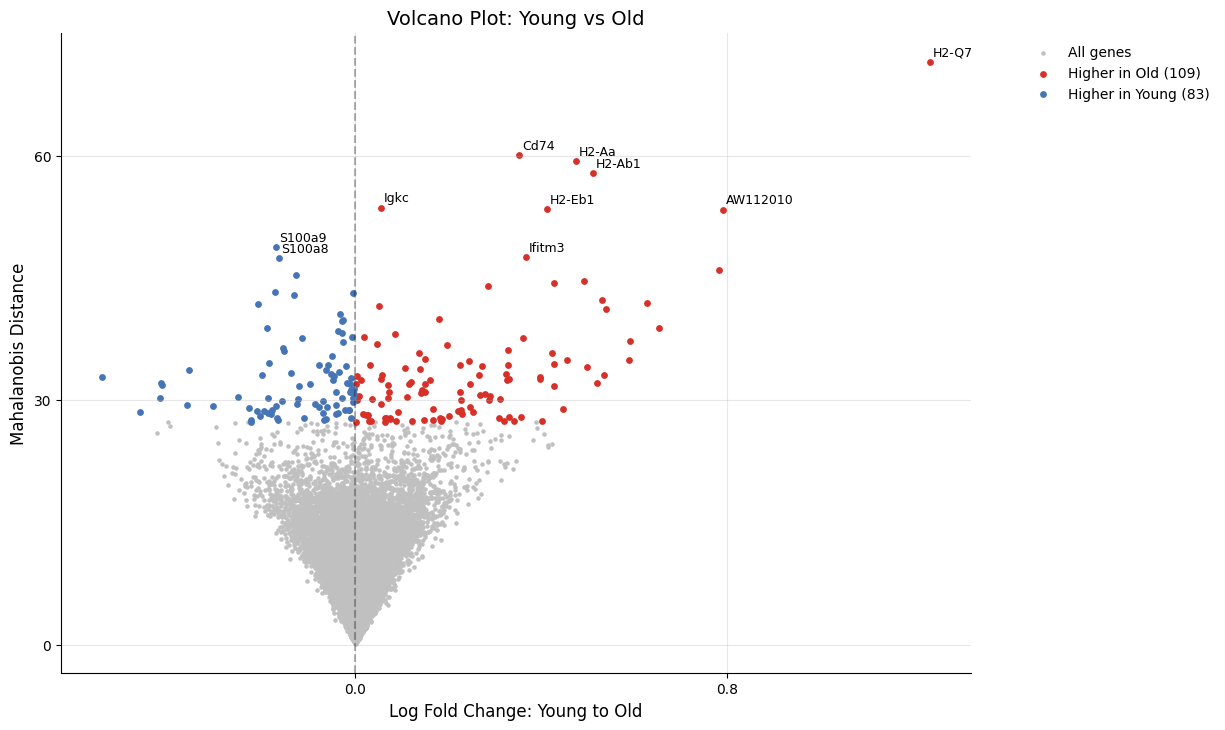
Volcano Plot¶

Visualize effect size vs. significance for differential expression with the volcano_de plot:

[15]:

kompot.plot.volcano_de(adata)

[2026-03-26 05:07:26,577] [INFO    ] Found DE run info for run_id=-1
[2026-03-26 05:07:26,578] [INFO    ] Found mean_lfc_key='kompot_de_Young_to_Old_mean_lfc' from run info
[2026-03-26 05:07:26,579] [INFO    ] Found mahalanobis_key='kompot_de_Young_to_Old_mahalanobis' from run info
[2026-03-26 05:07:26,580] [INFO    ] Successfully inferred fields: {'mean_lfc_key': 'kompot_de_Young_to_Old_mean_lfc', 'mahalanobis_key': 'kompot_de_Young_to_Old_mahalanobis'}
[2026-03-26 05:07:26,581] [INFO    ] Using DE run 0: comparing Young to Old
[2026-03-26 05:07:26,598] [INFO    ] Using data columns from var - lfc: 'kompot_de_Young_to_Old_mean_lfc', score: 'kompot_de_Young_to_Old_mahalanobis'
[2026-03-26 05:07:26,602] [INFO    ] Highlighting 192 genes marked as DE (109 up, 83 down)
[2026-03-26 05:07:26,614] [INFO    ] Labeling top 10 genes by score

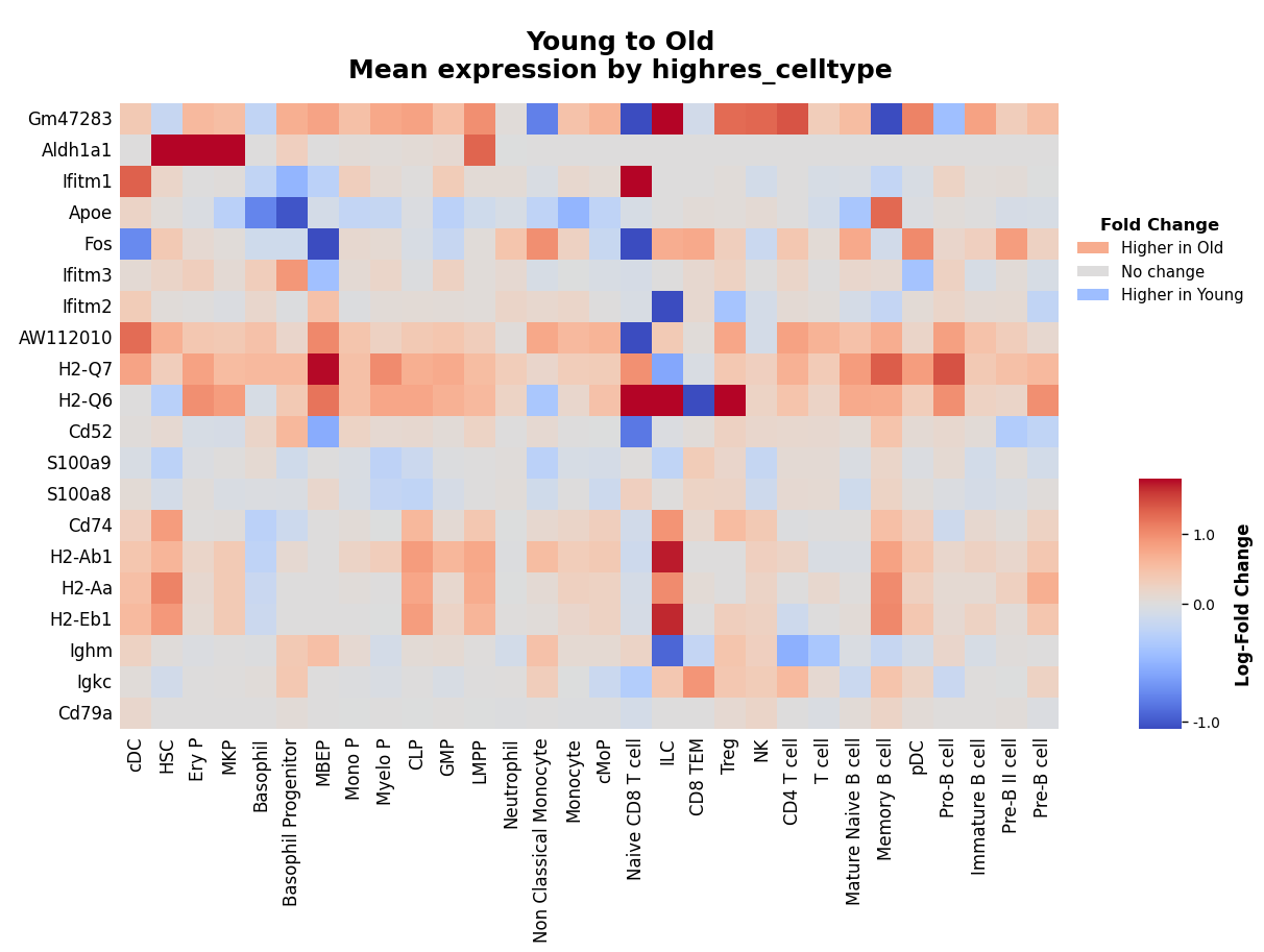
../_images/notebooks_01_getting_started_30_1.png

Fold Change Heatmap¶

Visualize fold changes across top differentially expressed genes with a heatmap. This provides a complementary view to the volcano plot, showing the magnitude and direction of expression changes.

Note that the gene selection is based on Kompot’s Mahalanobis distance (statistical significance), but the fold changes displayed are simply the difference of mean expressions from the input expression layer (in this case logged_counts), not a Kompot-specific metric:

[16]:

# Selecting top 20 genes
genes = adata.var[f"kompot_de_{CONDITIONS[0]}_to_{CONDITIONS[1]}_mahalanobis"].sort_values(ascending=False).head(20).index

kompot.plot.heatmap(
    adata,
    genes=genes,
    groupby=CELL_TYPE_COLUMN,        # Aggregate expression by cell type
    exclude_groups="Plasma cell",    # Remove cell types with too little representation
    vmin="p1",                       # Color scale minimum at 1st percentile (handles outliers)
    vmax="p99",                      # Color scale maximum at 99th percentile
    fold_change_mode=True,           # Display fold changes instead of mean expression
)

[2026-03-26 05:07:26,879] [INFO    ] Inferred condition_column='Age' from run information
[2026-03-26 05:07:26,880] [INFO    ] Inferred condition1='Young' from run information
[2026-03-26 05:07:26,881] [INFO    ] Inferred condition2='Old' from run information
[2026-03-26 05:07:26,882] [INFO    ] Inferred layer='logged_counts' from run information
[2026-03-26 05:07:26,883] [INFO    ] Creating fold change heatmap with 20 genes/features
[2026-03-26 05:07:26,885] [INFO    ] Using expression data from layer: 'logged_counts'
[2026-03-26 05:07:26,958] [INFO    ] Excluded 7 cells from groups: Plasma cell
[2026-03-26 05:07:26,965] [INFO    ] Applying gene-wise z-scoring (standard_scale='var')
[2026-03-26 05:07:27,037] [WARNING ] standard_scale is ignored in fold_change_mode as z-scoring is not appropriate for fold changes

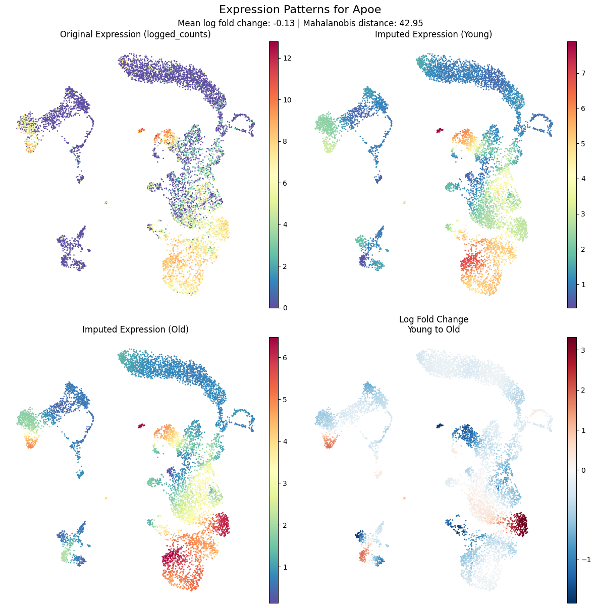
../_images/notebooks_01_getting_started_32_1.png

[21]:

kompot.plot.plot_gene_expression(
    adata, gene="Apoe", frameon=False
)

[2026-03-27 01:03:17,660] [INFO    ] Found DE run info for run_id=-1
[2026-03-27 01:03:17,662] [INFO    ] Found mean_lfc_key='kompot_de_Young_to_Old_mean_lfc' from run info
[2026-03-27 01:03:17,664] [INFO    ] Found mahalanobis_key='kompot_de_Young_to_Old_mahalanobis' from run info
[2026-03-27 01:03:17,666] [INFO    ] Successfully inferred fields: {'mean_lfc_key': 'kompot_de_Young_to_Old_mean_lfc', 'mahalanobis_key': 'kompot_de_Young_to_Old_mahalanobis'}
[2026-03-27 01:03:17,667] [INFO    ] Using DE run 0: comparing Young to Old
[2026-03-27 01:03:17,669] [INFO    ] Using fields for gene expression plot - lfc_key: 'kompot_de_Young_to_Old_mean_lfc', score_key: 'kompot_de_Young_to_Old_mahalanobis'
[2026-03-27 01:03:17,670] [INFO    ] Using layer 'logged_counts' inferred from run information
[2026-03-27 01:03:17,673] [INFO    ] Using imputed layer 'kompot_de_Young_imputed' for 'Young'
[2026-03-27 01:03:17,674] [INFO    ] Using imputed layer 'kompot_de_Old_imputed' for 'Old'
[2026-03-27 01:03:17,674] [INFO    ] Using fold_change layer 'kompot_de_Young_to_Old_fold_change' from run_info

../_images/notebooks_01_getting_started_33_1.png

Functional Enrichment¶

Use StringDBReport to analyze gene sets using STRING database:

Privacy Note: This sends gene lists to the STRING database API. If working with sensitive data, consider local alternatives.

[ ]:

# Selecting all significantly different genes
genes = adata.var_names[adata.var[f"kompot_de_{CONDITIONS[0]}_to_{CONDITIONS[1]}_is_de"]]

# Create STRING report
report = kompot.plot.StringDBReport(
    genes,
    species_id=10090, # 10090 = Mus musculus, 9606 = Homo Sapiens
    include_enrichment=True
)
report

[19]:

# Get enriched functional categories
report.get_functional_enrichment("Function").head(10)

[19]:

	category	term	number_of_genes	number_of_genes_in_background	ncbiTaxonId	inputGenes	preferredNames	p_value	fdr	description	expected	strength	signal
774	Function	GO:0042605	10	31	10090	[H2-K1, H2-Ab1, H2-Aa, H2-Q7, H2-T22, H2-Q4, H...	[H2-K1, H2-Ab1, H2-Aa, H2-Q7, H2-T22, H2-Q4, H...	1.600000e-12	3.910000e-09	Peptide antigen binding	0.281818	1.550031	0.899806
772	Function	GO:0003823	12	63	10090	[H2-K1, H2-Ab1, H2-Aa, H2-Q7, H2-T22, H2-Q4, H...	[H2-K1, H2-Ab1, H2-Aa, H2-Q7, H2-T22, H2-Q4, H...	1.940000e-12	3.910000e-09	Antigen binding	0.572727	1.321233	0.680418
777	Function	GO:0042608	8	31	10090	[H2-K1, H2-Q7, H2-T22, H2-Q4, H2-T23, Lck, H2-...	[H2-K1, H2-Q7, H2-T22, H2-Q4, H2-T23, Lck, H2-...	1.290000e-09	9.050000e-07	T cell receptor binding	0.281818	1.453121	0.678800
780	Function	GO:0042610	7	24	10090	[H2-K1, H2-Q7, H2-T22, H2-Q4, H2-T23, Lck, H2-Q6]	[H2-K1, H2-Q7, H2-T22, H2-Q4, H2-T23, Lck, H2-Q6]	7.010000e-09	3.440000e-06	CD8 receptor binding	0.218182	1.506279	0.672675
782	Function	GO:0046979	7	25	10090	[H2-K1, H2-Q7, H2-T22, H2-Q4, H2-T23, Tap1, H2...	[H2-K1, H2-Q7, H2-T22, H2-Q4, H2-T23, Tap1, H2...	8.910000e-09	3.920000e-06	TAP2 binding	0.227273	1.488551	0.657889
783	Function	GO:0046978	7	26	10090	[H2-K1, H2-Q7, H2-T22, H2-Q4, H2-T23, Tap1, H2...	[H2-K1, H2-Q7, H2-T22, H2-Q4, H2-T23, Tap1, H2...	1.120000e-08	4.230000e-06	TAP1 binding	0.236364	1.471517	0.645364
775	Function	GO:0042287	10	52	10090	[H2-K1, Cd81, Cd8b1, H2-Q7, H2-T22, H2-Q4, Cd7...	[H2-K1, Cd81, Cd8b1, H2-Q7, H2-T22, H2-Q4, Cd7...	1.310000e-10	1.280000e-07	MHC protein binding	0.472727	1.325389	0.628116
781	Function	GO:0042288	8	41	10090	[H2-K1, Cd8b1, H2-Q7, H2-T22, H2-Q4, H2-T23, T...	[H2-K1, Cd8b1, H2-Q7, H2-T22, H2-Q4, H2-T23, T...	8.800000e-09	3.920000e-06	MHC class I protein binding	0.372727	1.331699	0.562132
788	Function	GO:0030881	6	25	10090	[H2-K1, H2-Q7, H2-T22, H2-Q4, H2-T23, H2-Q6]	[H2-K1, H2-Q7, H2-T22, H2-Q4, H2-T23, H2-Q6]	2.340000e-07	6.040000e-05	beta-2-microglobulin binding	0.227273	1.421604	0.532037
786	Function	GO:0071889	8	55	10090	[Zfp36l1, H2-K1, Zfp36, H2-Q7, H2-T22, H2-Q4, ...	[Zfp36l1, H2-K1, Zfp36, H2-Q7, H2-T22, H2-Q4, ...	6.820000e-08	1.970000e-05	14-3-3 protein binding	0.500000	1.204120	0.452814

Inspecting Run History with RunInfo¶

Kompot tracks the history of all differential analysis runs, including parameters, environment, and results. The RunInfo class provides easy access to this information:

See kompot.RunInfo for full documentation.

[20]:

# Get info about the most recent DE run
de_run = kompot.RunInfo(adata, analysis_type='de')
de_run

[20]:

Run 0 (DE Analysis)

Run Summary

Analysis: DE | Run ID: 0 | Timestamp: 2026-03-26T05:07:26.115269 | Conditions: Young to OldAll Fields Present

Parameter	Value
conditions	Young to Old
obsm_key	DM_EigenVectors
uses_sample_variance	False
layer	logged_counts
timestamp	2026-03-26T05:07:26.115269
Fields Created	9

All Parameters

Parameter	Value
auto_filtered	False
batch_size	0
compute_mahalanobis	True
condition1	Young
condition2	Old
copy	False
eps	1e-08
fdr_threshold	0.05
groupby	Age
inplace	True
jit_compile	False
landmarks	False
layer	logged_counts
ls_factor	10.0
max_memory_ratio	0.8
min_cells	2
n_landmarks	5000
null_genes	2000
null_seed	42
obsm_key	DM_EigenVectors
result_key	kompot_de
sigma	1.0
store_landmarks	False
store_posterior_covariance	False
use_empirical_variance	False
use_sample_variance	False
used_landmarks	False

Environment

Parameter	Value
hostname	gizmok39
package_versions	anndata: 0.12.10 jax: 0.9.0.1 jaxlib: 0.9.0.1 kompot: 0.7.0 numpy: 2.4.2 pandas: 2.3.3 scipy: 1.17.1
pid	23834
platform	Linux-4.15.0-213-generic-x86_64-with-glibc2.35
python_version	3.12.12
timestamp	2026-03-26T05:07:26.142933
username	dotto

Fields Created by This Run

Total Fields: 9 | Present: 9 | Missing: 0 | Overwritten: 0

Field Name	Location	Description	Status
LAYERS Fields
kompot_de_Old_imputed	layers	[imputed] Imputed expression for Old	Present
kompot_de_Young_imputed	layers	[imputed] Imputed expression for Young	Present
kompot_de_Young_to_Old_fold_change	layers	[fold_change] Log fold change for each cell and gene	Present
OBS Fields
kompot_de_Old_std	obs	[std] Posterior standard deviation of imputed expression for Old (same for all genes)	Present
kompot_de_Young_std	obs	[std] Posterior standard deviation of imputed expression for Young (same for all genes)	Present
VAR Fields
kompot_de_Young_to_Old_is_de	var	[is_de] Boolean indicator of differential expression at local FDR < 0.05	Present
kompot_de_Young_to_Old_mahalanobis	var	[mahalanobis] Mahalanobis distances	Present
kompot_de_Young_to_Old_mahalanobis_local_fdr	var	[mahalanobis_local_fdr] Local FDR values using empirical null estimation similar to R's fdrtool	Present
kompot_de_Young_to_Old_mean_lfc	var	[mean_log_fold_change] Mean log fold change values	Present

Saving Results¶

Optional: Cleanup Large Layers¶

Imputed expression layers can be large. Remove them if not needed for further analysis with the cleanup utility:

[21]:

kompot.cleanup(adata)

[2026-03-26 05:08:11,132] [INFO    ] Cleaning up all 1 run(s)
[2026-03-26 05:08:11,144] [INFO    ] Cleaned up 3 field(s) from run 0:
[2026-03-26 05:08:11,145] [INFO    ]   layers (3 field(s)):
[2026-03-26 05:08:11,146] [INFO    ]     - kompot_de_Young_imputed
[2026-03-26 05:08:11,147] [INFO    ]     - kompot_de_Old_imputed
[2026-03-26 05:08:11,148] [INFO    ]     - kompot_de_Young_to_Old_fold_change
[2026-03-26 05:08:11,149] [INFO    ] Total: Cleaned up 3 field(s) across 1 run(s)

This removes:

kompot_de_Young_imputed
kompot_de_Old_imputed
kompot_de_Young_to_Old_fold_change

Statistical results in adata.var and adata.obs are preserved.

[22]:

adata.write_h5ad("../data/murine_bone_marrow_aging_processed.h5ad")

Biological Interpretation¶

Key Findings¶

Differential Abundance:

HSCs show increased abundance in Old mice
Naive CD8 T cells are predominantly Young
Consistent with age-related HSC expansion and T cell depletion

Differential Expression:

MHC class II genes (H2-Q7, Cd74, H2-Aa, H2-Ab1): Upregulated in Old mice → enhanced antigen presentation
Antioxidant genes (S100a8, S100a9, Apoe): Higher in Young → reduced oxidative stress
Interferon-stimulated genes (Ifitm family): Age-related changes in immune response

These patterns suggest aging leads to chronic immune activation (“inflammaging”) and altered stem cell dynamics.

Next Steps¶

Tutorial 2: Differential Expression Deep Dive - Advanced DE analysis options
Tutorial 3: Sample Variance Analysis - Account for biological replicates

For complete documentation, visit kompot.readthedocs.io