Estimating Expression Functions with smooth_expression

kompot.smooth_expression fits a Gaussian process over the cell-state embedding to turn noisy per-cell counts into a smooth expression function f(state) — plus per-cell uncertainty, of which there are two distinct kinds: how well-determined the function is (the GP posterior standard deviation, driven by where cells are) and how far the measurements themselves scatter around it (the empirical variance, driven by the gene). Section 2 separates them.

This is the same machinery that kompot.de uses internally: differential expression fits one of these functions per condition and contrasts them. Using the primitive directly unlocks two things DE wraps up: reading the uncertainties, and training on some cells then predicting on others (imputation, modality transfer, counterfactual expression).

We start with the plainest possible call and add one idea at a time.

Dive deeper: Getting Started / DE · Advanced DE and ls_factor · Sample variance · Paper

%matplotlib inline

import os
import anndata as ad
import matplotlib.pyplot as plt
import numpy as np
import scanpy as sc
from scipy import sparse

import kompot

# Consistent, clean plotting style across the tutorial set
plt.rcParams["axes.spines.right"] = False
plt.rcParams["axes.spines.top"] = False
plt.rcParams["image.cmap"] = "Spectral_r"

os.environ["LOKY_MAX_CPU_COUNT"] = "8"

/fh/fast/setty_m/user/dotto/nexus/work/kompot-080/.venv-312/lib/python3.12/site-packages/tqdm/auto.py:21: TqdmWarning: IProgress not found. Please update jupyter and ipywidgets. See https://ipywidgets.readthedocs.io/en/stable/user_install.html
  from .autonotebook import tqdm as notebook_tqdm

Configuration

Same dataset and cell-state representation as the DE tutorials:

DATA_PATH = "../data/murine_bone_marrow_aging.h5ad"
GROUPING_COLUMN = "Age"                       # condition column in adata.obs
CONDITIONS = ["Young", "Old"]                 # first entry is the reference
CELL_TYPE_COLUMN = "highres_celltype"         # for visualization only
DIMENSIONALITY_REDUCTION = "DM_EigenVectors"  # cell-state representation
LAYER_FOR_EXPRESSION = "logged_counts"        # expression layer

# A few lineage markers to smooth (myeloid, B, erythroid programs).
GENES = ["Elane", "Mpo", "Cd79a", "Car2"]


def dense(x):
    return np.asarray(x.todense()).ravel() if sparse.issparse(x) else np.asarray(x).ravel()

Load Data

import os
from pathlib import Path

import requests
from tqdm.auto import tqdm

Path(DATA_PATH).parent.mkdir(parents=True, exist_ok=True)

if not os.path.exists(DATA_PATH):
    print("Downloading dataset (~2.4 GB) from Zenodo ...")
    url = "https://zenodo.org/records/15587768/files/murine_bone_marrow_aging.h5ad?download=1"
    response = requests.get(url, stream=True)
    total = int(response.headers.get("content-length", 0))
    with open(DATA_PATH, "wb") as file, tqdm(total=total, unit="B", unit_scale=True) as bar:
        for chunk in response.iter_content(chunk_size=1 << 20):
            file.write(chunk)
            bar.update(len(chunk))

adata = ad.read_h5ad(DATA_PATH)
adata

AnnData object with n_obs × n_vars = 8090 × 16285
    obs: 'Compartment', 'Replicate', 'Age', 'Sample', 'Info', 'batch', 'doublet_score', 'n_genes_by_counts', 'total_counts', 'total_counts_mt', 'pct_counts_mt', 'total_counts_hb', 'pct_counts_hb', 'S_score', 'G2M_score', 'phase', 'leiden', 'phenograph', 'highres_celltype', 'midres_celltype'
    var: 'gene_ids', 'feature_types', 'genome', 'mt', 'n_cells_by_counts', 'mean_counts', 'pct_dropout_by_counts', 'total_counts', 'hb', 'highly_variable', 'means', 'dispersions', 'dispersions_norm', 'highly_variable_nbatches', 'highly_variable_intersection'
    uns: 'Age_colors', 'Compartment_colors', 'DMEigenValues', 'DM_EigenValues', 'Info_colors', 'README', 'Replicate_colors', 'Sample_colors', 'batch_colors', 'draw_graph', 'highres_celltype_colors', 'hvg', 'leiden', 'leiden_colors', 'midres_celltype_colors', 'neighbors', 'pca', 'phase_colors', 'umap'
    obsm: 'AbCapture', 'DM_EigenVectors', 'HTO', 'X_draw_graph_fa', 'X_pca', 'X_pca_harmony', 'X_pca_noregression', 'X_umap'
    varm: 'PCs'
    obsp: 'DM_Kernel', 'DM_Similarity', 'connectivities', 'distances'
    layers: 'MAGIC_imputed_data', 'cc_counts', 'logged_counts', 'normalized_counts', 'raw_counts', None (.X)

1. The vanilla case

Fit an expression function on all cells. Give it the cell-state representation, the expression layer, and the genes you care about — that is the whole call:

kompot.smooth_expression(
    adata,
    obsm_key=DIMENSIONALITY_REDUCTION,
    layer=LAYER_FOR_EXPRESSION,
    genes=GENES,
)

smoothed = "kompot_smooth_all_smoothed"   # layer: the fitted function, per cell
std = "kompot_smooth_all_std"             # layer: its posterior standard deviation

adata

An NVIDIA GPU may be present on this machine, but a CUDA-enabled jaxlib is not installed. Falling back to cpu.

[2026-07-28 13:27:22,869] [INFO    ] Smoothing all 8,090 cells

Predicting expression: 100%|██████████| 17/17 [00:01<00:00,  9.54it/s]
Computing GP covariance (diag): 100%|██████████| 17/17 [00:08<00:00,  1.94it/s]

AnnData object with n_obs × n_vars = 8090 × 16285
    obs: 'Compartment', 'Replicate', 'Age', 'Sample', 'Info', 'batch', 'doublet_score', 'n_genes_by_counts', 'total_counts', 'total_counts_mt', 'pct_counts_mt', 'total_counts_hb', 'pct_counts_hb', 'S_score', 'G2M_score', 'phase', 'leiden', 'phenograph', 'highres_celltype', 'midres_celltype'
    var: 'gene_ids', 'feature_types', 'genome', 'mt', 'n_cells_by_counts', 'mean_counts', 'pct_dropout_by_counts', 'total_counts', 'hb', 'highly_variable', 'means', 'dispersions', 'dispersions_norm', 'highly_variable_nbatches', 'highly_variable_intersection'
    uns: 'Age_colors', 'Compartment_colors', 'DMEigenValues', 'DM_EigenValues', 'Info_colors', 'README', 'Replicate_colors', 'Sample_colors', 'batch_colors', 'draw_graph', 'highres_celltype_colors', 'hvg', 'leiden', 'leiden_colors', 'midres_celltype_colors', 'neighbors', 'pca', 'phase_colors', 'umap', 'kompot_smooth'
    obsm: 'AbCapture', 'DM_EigenVectors', 'HTO', 'X_draw_graph_fa', 'X_pca', 'X_pca_harmony', 'X_pca_noregression', 'X_umap'
    varm: 'PCs'
    obsp: 'DM_Kernel', 'DM_Similarity', 'connectivities', 'distances'
    layers: 'MAGIC_imputed_data', 'cc_counts', 'logged_counts', 'normalized_counts', 'raw_counts', None (.X), 'kompot_smooth_all_smoothed', 'kompot_smooth_all_std'

Two new layers. The raw counts are noisy and full of dropouts; the fitted function denoises them into a smooth surface over cell state, and the posterior std says how much to trust it at each cell. Look at all three for one gene:

gene = GENES[0]
gi = adata.var_names.get_loc(gene)

adata.obs[f"{gene}: raw"] = dense(adata[:, gene].layers[LAYER_FOR_EXPRESSION])
adata.obs[f"{gene}: smoothed"] = adata.layers[smoothed][:, gi]
adata.obs[f"{gene}: posterior std"] = adata.layers[std][:, gi]

fig, axes = plt.subplots(1, 3, figsize=(12, 3.6))
sc.pl.embedding(adata, "umap", color=f"{gene}: raw", ax=axes[0], show=False,
                frameon=False, cmap="Spectral_r")
sc.pl.embedding(adata, "umap", color=f"{gene}: smoothed", ax=axes[1],
                show=False, frameon=False, cmap="Spectral_r")
sc.pl.embedding(adata, "umap", color=f"{gene}: posterior std", ax=axes[2],
                show=False, frameon=False, cmap="magma")
plt.tight_layout()

2. Two kinds of uncertainty

The _std layer above is the GP posterior standard deviation: how well-determined the expression function is at each cell. It is driven by cell availability — tight where the embedding is densely sampled, wide where cells are sparse or the fit is extrapolating.

It is worth being precise about what that number does not contain. With only the GP covariance in play it depends on the cell-state geometry alone — on where cells sit, not on what was measured in them — so it is the same for every gene. Kompot computes one column and broadcasts it across genes, which the next cell verifies directly. It therefore says nothing about a gene being noisy, lowly expressed, or bursty: it is purely the availability-of-cells part of the uncertainty, and it ignores any variability that depends on expression level.

The missing half is the variability of the measurements themselves — how far individual counts scatter around the fitted function. That is gene-specific and expression-dependent, and it is what use_empirical_variance=True estimates, adding an _obs_variance layer: leverage-corrected squared residuals smoothed by a second GP into an input-dependent noise surface.

The two answer different questions, and the difference is practical:

	question	shrinks with more cells?	gene-specific?
_std (posterior)	where is the function?	yes	no
_obs_variance (empirical)	how far do measurements scatter around it?	no	yes

Collecting more cells makes the first shrink and leaves the second alone — scatter is a property of the biology and the assay, not of how much of it you sampled. A gene can have a confidently placed function that individual cells still scatter widely around, and reading the posterior std alone would call that gene well-behaved.

Since 0.8.0 use_empirical_variance defaults to False everywhere, so this is opt-in.

from kompot import GPSettings, OutputSettings, StorageSettings

# The posterior std carries no gene-specific information: verify it directly.
gene_cols = [adata.var_names.get_loc(g) for g in GENES]
stds = adata.layers[std][:, gene_cols]
print("posterior std identical across genes:",
      np.allclose(stds, stds[:, :1], equal_nan=True))

# Re-fit asking for the empirical (measurement) variability as well.
kompot.smooth_expression(
    adata,
    obsm_key=DIMENSIONALITY_REDUCTION,
    layer=LAYER_FOR_EXPRESSION,
    genes=GENES,
    gp=GPSettings(use_empirical_variance=True),
    storage=StorageSettings(result_key="kompot_smooth_emp"),
    output=OutputSettings(progress=False),
)

obs_var = "kompot_smooth_emp_all_obs_variance"   # layer: measurement variability

adata.obs[f"{gene}: obs sd"] = np.sqrt(adata.layers[obs_var][:, gi])

fig, axes = plt.subplots(1, 3, figsize=(12, 3.6))
sc.pl.embedding(adata, "umap", color=f"{gene}: smoothed", ax=axes[0], show=False,
                frameon=False, cmap="Spectral_r", title="fitted function")
sc.pl.embedding(adata, "umap", color=f"{gene}: posterior std", ax=axes[1], show=False,
                frameon=False, cmap="magma", title="posterior std (cell availability)")
sc.pl.embedding(adata, "umap", color=f"{gene}: obs sd", ax=axes[2], show=False,
                frameon=False, cmap="viridis", title="empirical sd (measurement scatter)")
plt.tight_layout()

posterior std identical across genes: True
[2026-07-28 13:28:26,517] [INFO    ] Smoothing all 8,090 cells

That is the primitive: a denoised expression function and a calibrated uncertainty on the same cell-state geometry. Uncertainty is highest where cells are sparse — the model tells you where it is guessing.

Everything below is the same call with one knob turned.

3. The length scale

The length scale sets how far the GP pools information across neighbouring cells. GPSettings(ls_factor=...) scales the automatically inferred length scale (default 10). Fit the same gene at a low, medium, and high ls_factor and read the smoothed value (top) against its posterior std (bottom):

scales = [(1.0, "sharp"), (10.0, "default"), (100.0, "smooth")]
X = adata.obsm[DIMENSIONALITY_REDUCTION]
gj = GENES.index(gene)

fig, axes = plt.subplots(2, len(scales), figsize=(4 * len(scales), 7))
for k, (lsf, tag) in enumerate(scales):
    model = kompot.smooth_expression(
        adata,
        obsm_key=DIMENSIONALITY_REDUCTION, layer=LAYER_FOR_EXPRESSION, genes=GENES,
        gp=kompot.GPSettings(ls_factor=lsf),
        storage=kompot.StorageSettings(result_key=f"ls_{tag}"),
        output=kompot.OutputSettings(return_full_results=True, inplace=False, progress=False),
    )["model"]
    values = model.predict(X, progress=False)[:, gj]
    sd = model.std(X, progress=False)
    sd = sd[:, gj] if sd.ndim == 2 else sd.ravel()

    adata.obs["_value"], adata.obs["_sd"] = values, sd
    sc.pl.embedding(adata, "umap", color="_value", ax=axes[0, k], show=False, vmin=0, vmax=3,
                    frameon=False, cmap="Spectral_r", title=f"ls_factor={lsf:g} ({tag})")
    sc.pl.embedding(adata, "umap", color="_sd", ax=axes[1, k], show=False,
                    frameon=False, cmap="magma",
                    title=f"posterior std (mean {sd.mean():.3f})")
adata.obs.drop(columns=["_value", "_sd"], inplace=True)
plt.tight_layout()

[2026-07-28 13:30:22,745] [INFO    ] Smoothing all 8,090 cells
[2026-07-28 13:31:55,722] [INFO    ] Smoothing all 8,090 cells
[2026-07-28 13:33:28,261] [INFO    ] Smoothing all 8,090 cells

Larger ls_factor → a smoother surface with lower posterior uncertainty, at the cost of coarser resolution (fine structure is averaged away); smaller ls_factor does the reverse. That is the resolution–uncertainty trade-off. The Advanced DE tutorial covers ls_factor in the DE setting.

4. Fit on some cells, predict on others

The model is fit on the cells you give it but can be evaluated at any coordinates, so it doubles as a fit/predict surface. The bare-array estimator underneath smooth_expression is ExpressionModel:

• ExpressionModel().fit(X, y) — learn the function from cell-state coordinates X (n_cells, n_dims) and values y (n_cells, n_features).

• .predict(X) / .std(X) — evaluate the function and its uncertainty at any coordinates.

• .predictor.gradient(X) - evaluate the gradient of the function.

Imputing a sparsely measured modality

When a measurement exists on only some cells (a surface-protein panel, a spatial readout, a second assay), the same GP transfers it to the rest.

To grade the transfer honestly, take a real gene, hide it on a random 50% of cells, fit on the rest, and impute the hidden ones. Random cells are the right hold-out here: they are interspersed among measured cells, so every imputed cell has observed neighbours. That is the realistic modality-transfer regime. (Blanking one contiguous region instead would ask the model to extrapolate into states it has no representatives for — a different and much harder problem, and one the posterior std would correctly flag as unreliable.)

Because we hid real measurements, the ground truth is available to score against — a built-in cross-validation.

truth = dense(adata[:, gene].layers[LAYER_FOR_EXPRESSION])   # full, pre-masking
X = adata.obsm[DIMENSIONALITY_REDUCTION]

rng = np.random.default_rng(0)                               # seeded: reproducible
missing = rng.random(adata.n_obs) < 0.50                     # 50% of cells, at random
observed = ~missing

measured = truth.copy()
measured[missing] = np.nan                                   # the modality, on ~50% of cells

# Bare-array fit/predict — the estimator underneath smooth_expression.
model = kompot.ExpressionModel()
model.fit(X[observed], measured[observed][:, None])          # train on measured cells only

completed = measured.copy()                                  # measured cells keep their value
completed[missing] = model.predict(X[missing], progress=False)[:, 0]   # the rest are imputed

adata.obs[f"{gene}: measured (50% blanked)"] = measured
adata.obs[f"{gene}: completed (imputed)"] = completed
print(f"imputed {int(missing.sum())} cells from {int(observed.sum())} measured cells")

imputed 4057 cells from 4033 measured cells

The masked cells are scattered everywhere (grey), not carved out of one region; the completed layer fills them in from the shared cell-state geometry:

vmin, vmax = np.nanmin(truth), np.nanmax(truth)
fig, axes = plt.subplots(1, 2, figsize=(9, 3.8))
sc.pl.embedding(adata, "umap", color=f"{gene}: measured (50% blanked)", ax=axes[0],
                show=False, frameon=False, cmap="Spectral_r", vmin=vmin, vmax=vmax,
                na_color="lightgrey", title=f"{gene}: measured (blanked = grey)")
sc.pl.embedding(adata, "umap", color=f"{gene}: completed (imputed)", ax=axes[1],
                show=False, frameon=False, cmap="Spectral_r", vmin=vmin, vmax=vmax,
                title=f"{gene}: completed (imputed)")
plt.tight_layout()

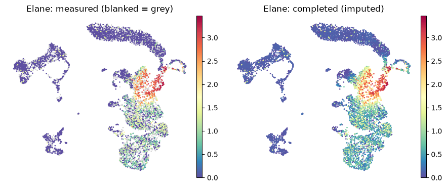
Now grade it against the truth we hid. Two populations tell two different stories — the imputed cells (never seen during the fit) and the smoothed input cells (denoised training values) — so we report a separate correlation for each:

pred_imputed = model.predict(X[missing], progress=False)[:, 0]    # held-out cells
pred_smoothed = model.predict(X[observed], progress=False)[:, 0]  # training cells

r_imputed = np.corrcoef(pred_imputed, truth[missing])[0, 1]
r_smoothed = np.corrcoef(pred_smoothed, truth[observed])[0, 1]

fig, ax = plt.subplots(figsize=(5, 5))
ax.scatter(truth[observed], pred_smoothed, s=4, alpha=0.25, color="#4C72B0",
           label=f"input cells, smoothed  (r = {r_smoothed:.2f})")
ax.scatter(truth[missing], pred_imputed, s=4, alpha=0.40, color="#C44E52",
           label=f"held-out cells, imputed  (r = {r_imputed:.2f})")
lims = [float(np.nanmin(truth)), float(np.nanmax(truth))]
ax.plot(lims, lims, "k--", lw=1)
ax.set(xlabel=f"true {gene} (original, before masking)", ylabel="model estimate",
       title="Recovery vs. hidden ground truth")
ax.legend(loc="upper left", frameon=False, markerscale=3)
plt.tight_layout()

print(f"imputed  r = {r_imputed:.3f}")
print(f"smoothed r = {r_smoothed:.3f}")

imputed  r = 0.813
smoothed r = 0.825

The two correlations land in the same place: cells the model never saw are recovered as accurately as the training cells are denoised. That is the signature of a well-posed transfer — every held-out cell sits among measured neighbours, so the GP interpolates rather than extrapolates. If you instead hide a whole region of the manifold, the imputed correlation drops sharply and model.std(X) lights up over exactly those cells; the uncertainty is there to tell you which regime you are in.

The fitted model is reusable without refitting: ModelSettings(model1=model) injects it into smooth_expression or kompot.de to write imputed values into another AnnData.

5. Counterfactual expression

Fit the function on one condition, then evaluate it at other cells’ states: the result is what expression would be if those cells followed that condition’s program. Contrast the Young function against the Old function — their difference is exactly the log fold change kompot.de reports.

def condition_model(condition):
    return kompot.smooth_expression(
        adata, groupby=GROUPING_COLUMN, condition=condition,
        obsm_key=DIMENSIONALITY_REDUCTION, layer=LAYER_FOR_EXPRESSION, genes=GENES,
        output=kompot.OutputSettings(return_full_results=True, inplace=False, progress=False),
    )["model"]


young_fn = condition_model(CONDITIONS[0])
old_fn = condition_model(CONDITIONS[1])

young_pred = young_fn.predict(X, progress=False)[:, gj]   # counterfactual reference
old_pred = old_fn.predict(X, progress=False)[:, gj]

adata.obs[f"{gene}: Young fn (counterfactual)"] = young_pred
adata.obs[f"{gene}: Old fn (actual program)"] = old_pred
adata.obs[f"{gene}: Old - Young (log fold change)"] = old_pred - young_pred

fig, axes = plt.subplots(1, 3, figsize=(12, 3.6))
sc.pl.embedding(adata, "umap", color=f"{gene}: Young fn (counterfactual)", ax=axes[0],
                show=False, frameon=False, cmap="Spectral_r")
sc.pl.embedding(adata, "umap", color=f"{gene}: Old fn (actual program)", ax=axes[1],
                show=False, frameon=False, cmap="Spectral_r")
sc.pl.embedding(adata, "umap", color=f"{gene}: Old - Young (log fold change)", ax=axes[2],
                show=False, frameon=False, cmap="RdBu_r", vcenter=0)
plt.tight_layout()

[2026-07-28 13:35:22,975] [INFO    ] Smoothing condition 'Young': 2,917 cells
[2026-07-28 13:35:48,259] [INFO    ] Smoothing condition 'Old': 3,116 cells

That third panel is differential expression, computed by hand. kompot.de does this for every gene at once and adds the covariance-aware significance on top — see Getting Started.

Where to go deeper

• Getting Started / DE — the front door; smooth_expression is the primitive underneath.

• Advanced DE and ls_factor — the length-scale trade-off in the DE setting.

• DE with sample variance — per-gene aleatoric and replicate uncertainty (this tutorial shows the GP/epistemic term).

• Differential abundance — the same GP geometry applied to cell-state frequency.

• Paper · Documentation